盗墓笔记txt全集下载,手机推荐排行榜

主頁 > 知識庫 > PyTorch一小時掌握之神經(jīng)網(wǎng)絡氣溫預測篇

PyTorch一小時掌握之神經(jīng)網(wǎng)絡氣溫預測篇

概述

具體的案例描述在此就不多贅述. 同一數(shù)據(jù)集我們在機器學習里的隨機森林模型中已經(jīng)討論過.

導包

import numpy as np
import pandas as pd
import datetime
import matplotlib.pyplot as plt
from pandas.plotting import register_matplotlib_converters
from sklearn.preprocessing import StandardScaler
import torch

數(shù)據(jù)讀取

# ------------------1. 數(shù)據(jù)讀取------------------

# 讀取數(shù)據(jù)
data = pd.read_csv("temps.csv")

# 看看數(shù)據(jù)長什么樣子
print(data.head())

# 查看數(shù)據(jù)維度
print("數(shù)據(jù)維度:", data.shape)

# 產看數(shù)據(jù)類型
print("數(shù)據(jù)類型:", type(data))

輸出結果:
year month day week temp_2 temp_1 average actual friend
0 2016 1 1 Fri 45 45 45.6 45 29
1 2016 1 2 Sat 44 45 45.7 44 61
2 2016 1 3 Sun 45 44 45.8 41 56
3 2016 1 4 Mon 44 41 45.9 40 53
4 2016 1 5 Tues 41 40 46.0 44 41
數(shù)據(jù)維度: (348, 9)
數(shù)據(jù)類型: class 'pandas.core.frame.DataFrame'>

數(shù)據(jù)預處理

# ------------------2. 數(shù)據(jù)預處理------------------

# datetime 格式
dates = pd.PeriodIndex(year=data["year"], month=data["month"], day=data["day"], freq="D").astype(str)
dates = [datetime.datetime.strptime(date, "%Y-%m-%d") for date in dates]
print(dates[:5])

# 編碼轉換
data = pd.get_dummies(data)
print(data.head())

# 畫圖
plt.style.use("fivethirtyeight")
register_matplotlib_converters()

# 標簽
labels = np.array(data["actual"])

# 取消標簽
data = data.drop(["actual"], axis= 1)
print(data.head())

# 保存一下列名
feature_list = list(data.columns)

# 格式轉換
data_new = np.array(data)

data_new  = StandardScaler().fit_transform(data_new)
print(data_new[:5])

輸出結果:
[datetime.datetime(2016, 1, 1, 0, 0), datetime.datetime(2016, 1, 2, 0, 0), datetime.datetime(2016, 1, 3, 0, 0), datetime.datetime(2016, 1, 4, 0, 0), datetime.datetime(2016, 1, 5, 0, 0)]
year month day temp_2 ... week_Sun week_Thurs week_Tues week_Wed
0 2016 1 1 45 ... 0 0 0 0
1 2016 1 2 44 ... 0 0 0 0
2 2016 1 3 45 ... 1 0 0 0
3 2016 1 4 44 ... 0 0 0 0
4 2016 1 5 41 ... 0 0 1 0

[5 rows x 15 columns]
year month day temp_2 ... week_Sun week_Thurs week_Tues week_Wed
0 2016 1 1 45 ... 0 0 0 0
1 2016 1 2 44 ... 0 0 0 0
2 2016 1 3 45 ... 1 0 0 0
3 2016 1 4 44 ... 0 0 0 0
4 2016 1 5 41 ... 0 0 1 0

[5 rows x 14 columns]
[[ 0. -1.5678393 -1.65682171 -1.48452388 -1.49443549 -1.3470703
-1.98891668 2.44131112 -0.40482045 -0.40961596 -0.40482045 -0.40482045
-0.41913682 -0.40482045]
[ 0. -1.5678393 -1.54267126 -1.56929813 -1.49443549 -1.33755752
0.06187741 -0.40961596 -0.40482045 2.44131112 -0.40482045 -0.40482045
-0.41913682 -0.40482045]
[ 0. -1.5678393 -1.4285208 -1.48452388 -1.57953835 -1.32804474
-0.25855917 -0.40961596 -0.40482045 -0.40961596 2.47023092 -0.40482045
-0.41913682 -0.40482045]
[ 0. -1.5678393 -1.31437034 -1.56929813 -1.83484692 -1.31853195
-0.45082111 -0.40961596 2.47023092 -0.40961596 -0.40482045 -0.40482045
-0.41913682 -0.40482045]
[ 0. -1.5678393 -1.20021989 -1.8236209 -1.91994977 -1.30901917
-1.2198689 -0.40961596 -0.40482045 -0.40961596 -0.40482045 -0.40482045
2.38585576 -0.40482045]]

構建網(wǎng)絡模型

# ------------------3. 構建網(wǎng)絡模型------------------

x = torch.tensor(data_new)
y = torch.tensor(labels)

# 權重參數(shù)初始化
weights1 = torch.randn((14,128), dtype=float, requires_grad= True)
biases1 = torch.randn(128, dtype=float, requires_grad= True)
weights2 = torch.randn((128,1), dtype=float, requires_grad= True)
biases2 = torch.randn(1, dtype=float, requires_grad= True)

learning_rate = 0.001
losses = []

for i in range(1000):
    # 計算隱層
    hidden = x.mm(weights1) + biases1
    # 加入激活函數(shù)
    hidden = torch.relu(hidden)
    # 預測結果
    predictions = hidden.mm(weights2) + biases2
    # 計算損失
    loss = torch.mean((predictions - y) ** 2)

    # 打印損失值
    if i % 100 == 0:
        print("loss:", loss)
    # 反向傳播計算
    loss.backward()

    # 更新參數(shù)
    weights1.data.add_(-learning_rate * weights1.grad.data)
    biases1.data.add_(-learning_rate * biases1.grad.data)
    weights2.data.add_(-learning_rate * weights2.grad.data)
    biases2.data.add_(-learning_rate * biases2.grad.data)

    # 每次迭代清空
    weights1.grad.data.zero_()
    biases1.grad.data.zero_()
    weights2.grad.data.zero_()
    biases2.grad.data.zero_()

輸出結果:
loss: tensor(4746.8598, dtype=torch.float64, grad_fn=MeanBackward0>)
loss: tensor(156.5691, dtype=torch.float64, grad_fn=MeanBackward0>)
loss: tensor(148.9419, dtype=torch.float64, grad_fn=MeanBackward0>)
loss: tensor(146.1035, dtype=torch.float64, grad_fn=MeanBackward0>)
loss: tensor(144.5652, dtype=torch.float64, grad_fn=MeanBackward0>)
loss: tensor(143.5376, dtype=torch.float64, grad_fn=MeanBackward0>)
loss: tensor(142.7823, dtype=torch.float64, grad_fn=MeanBackward0>)
loss: tensor(142.2151, dtype=torch.float64, grad_fn=MeanBackward0>)
loss: tensor(141.7770, dtype=torch.float64, grad_fn=MeanBackward0>)
loss: tensor(141.4294, dtype=torch.float64, grad_fn=MeanBackward0>)

數(shù)據(jù)可視化

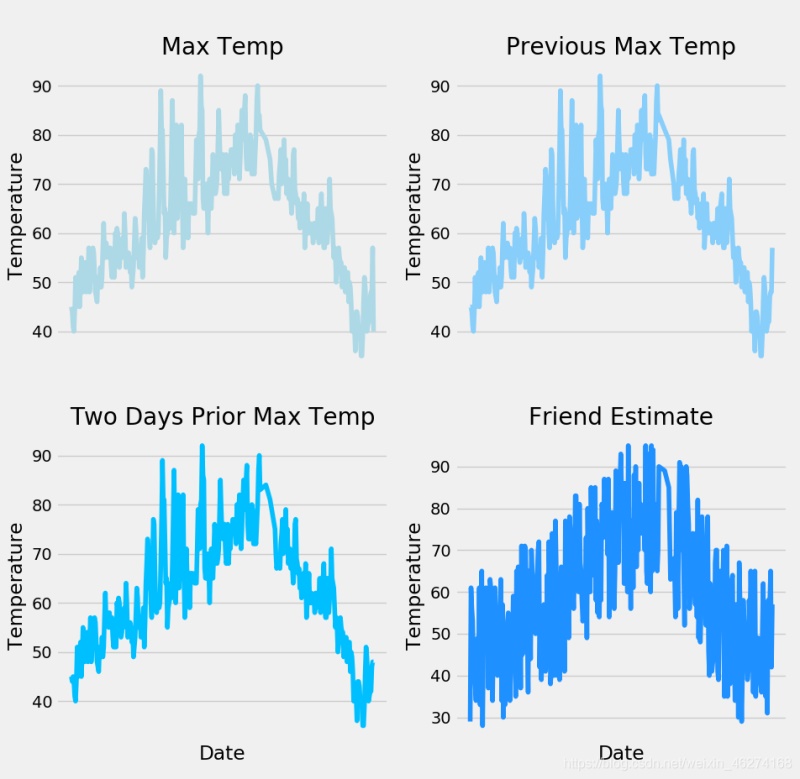
# ------------------4. 數(shù)據(jù)可視化------------------

def graph1():
    # 創(chuàng)建子圖
    f, ax = plt.subplots(2, 2, figsize=(10, 10))

    # 標簽值
    ax[0, 0].plot(dates, labels, color="#ADD8E6")
    ax[0, 0].set_xticks([""])
    ax[0, 0].set_ylabel("Temperature")
    ax[0, 0].set_title("Max Temp")

    # 昨天
    ax[0, 1].plot(dates, data["temp_1"], color="#87CEFA")
    ax[0, 1].set_xticks([""])
    ax[0, 1].set_ylabel("Temperature")
    ax[0, 1].set_title("Previous Max Temp")

    # 前天
    ax[1, 0].plot(dates, data["temp_2"], color="#00BFFF")
    ax[1, 0].set_xticks([""])
    ax[1, 0].set_xlabel("Date")
    ax[1, 0].set_ylabel("Temperature")
    ax[1, 0].set_title("Two Days Prior Max Temp")

    # 朋友
    ax[1, 1].plot(dates, data["friend"], color="#1E90FF")
    ax[1, 1].set_xticks([""])
    ax[1, 1].set_xlabel("Date")
    ax[1, 1].set_ylabel("Temperature")
    ax[1, 1].set_title("Friend Estimate")

    plt.show()

輸出結果:

完整代碼

import numpy as np
import pandas as pd
import datetime
import matplotlib.pyplot as plt
from pandas.plotting import register_matplotlib_converters
from sklearn.preprocessing import StandardScaler
import torch


# ------------------1. 數(shù)據(jù)讀取------------------

# 讀取數(shù)據(jù)
data = pd.read_csv("temps.csv")

# 看看數(shù)據(jù)長什么樣子
print(data.head())

# 查看數(shù)據(jù)維度
print("數(shù)據(jù)維度:", data.shape)

# 產看數(shù)據(jù)類型
print("數(shù)據(jù)類型:", type(data))

# ------------------2. 數(shù)據(jù)預處理------------------

# datetime 格式
dates = pd.PeriodIndex(year=data["year"], month=data["month"], day=data["day"], freq="D").astype(str)
dates = [datetime.datetime.strptime(date, "%Y-%m-%d") for date in dates]
print(dates[:5])

# 編碼轉換
data = pd.get_dummies(data)
print(data.head())

# 畫圖
plt.style.use("fivethirtyeight")
register_matplotlib_converters()

# 標簽
labels = np.array(data["actual"])

# 取消標簽
data = data.drop(["actual"], axis= 1)
print(data.head())

# 保存一下列名
feature_list = list(data.columns)

# 格式轉換
data_new = np.array(data)

data_new  = StandardScaler().fit_transform(data_new)
print(data_new[:5])

# ------------------3. 構建網(wǎng)絡模型------------------

x = torch.tensor(data_new)
y = torch.tensor(labels)

# 權重參數(shù)初始化
weights1 = torch.randn((14,128), dtype=float, requires_grad= True)
biases1 = torch.randn(128, dtype=float, requires_grad= True)
weights2 = torch.randn((128,1), dtype=float, requires_grad= True)
biases2 = torch.randn(1, dtype=float, requires_grad= True)

learning_rate = 0.001
losses = []

for i in range(1000):
    # 計算隱層
    hidden = x.mm(weights1) + biases1
    # 加入激活函數(shù)
    hidden = torch.relu(hidden)
    # 預測結果
    predictions = hidden.mm(weights2) + biases2
    # 計算損失
    loss = torch.mean((predictions - y) ** 2)

    # 打印損失值
    if i % 100 == 0:
        print("loss:", loss)
    # 反向傳播計算
    loss.backward()

    # 更新參數(shù)
    weights1.data.add_(-learning_rate * weights1.grad.data)
    biases1.data.add_(-learning_rate * biases1.grad.data)
    weights2.data.add_(-learning_rate * weights2.grad.data)
    biases2.data.add_(-learning_rate * biases2.grad.data)

    # 每次迭代清空
    weights1.grad.data.zero_()
    biases1.grad.data.zero_()
    weights2.grad.data.zero_()
    biases2.grad.data.zero_()

# ------------------4. 數(shù)據(jù)可視化------------------

def graph1():
    # 創(chuàng)建子圖
    f, ax = plt.subplots(2, 2, figsize=(10, 10))

    # 標簽值
    ax[0, 0].plot(dates, labels, color="#ADD8E6")
    ax[0, 0].set_xticks([""])
    ax[0, 0].set_ylabel("Temperature")
    ax[0, 0].set_title("Max Temp")

    # 昨天
    ax[0, 1].plot(dates, data["temp_1"], color="#87CEFA")
    ax[0, 1].set_xticks([""])
    ax[0, 1].set_ylabel("Temperature")
    ax[0, 1].set_title("Previous Max Temp")

    # 前天
    ax[1, 0].plot(dates, data["temp_2"], color="#00BFFF")
    ax[1, 0].set_xticks([""])
    ax[1, 0].set_xlabel("Date")
    ax[1, 0].set_ylabel("Temperature")
    ax[1, 0].set_title("Two Days Prior Max Temp")

    # 朋友
    ax[1, 1].plot(dates, data["friend"], color="#1E90FF")
    ax[1, 1].set_xticks([""])
    ax[1, 1].set_xlabel("Date")
    ax[1, 1].set_ylabel("Temperature")
    ax[1, 1].set_title("Friend Estimate")

    plt.show()


if __name__ == "__main__":
    graph1()

到此這篇關于PyTorch一小時掌握之神經(jīng)網(wǎng)絡氣溫預測篇的文章就介紹到這了,更多相關PyTorch 神經(jīng)網(wǎng)絡氣溫預測內容請搜索腳本之家以前的文章或繼續(xù)瀏覽下面的相關文章希望大家以后多多支持腳本之家！

您可能感興趣的文章:

PyTorch一小時掌握之autograd機制篇
PyTorch一小時掌握之神經(jīng)網(wǎng)絡分類篇
PyTorch一小時掌握之圖像識別實戰(zhàn)篇
PyTorch一小時掌握之基本操作篇

標簽：紹興吉安安康廣西蘭州懷化蕪湖呂梁

巨人網(wǎng)絡通訊聲明：本文標題《PyTorch一小時掌握之神經(jīng)網(wǎng)絡氣溫預測篇》，本文關鍵詞 PyTorch,一小時,掌握,之,神經(jīng)網(wǎng)絡,；如發(fā)現(xiàn)本文內容存在版權問題，煩請?zhí)峁┫嚓P信息告之我們，我們將及時溝通與處理。本站內容系統(tǒng)采集于網(wǎng)絡，涉及言論、版權與本站無關。

濮阳杆衣贸易有限公司

PyTorch一小時掌握之神經(jīng)網(wǎng)絡氣溫預測篇

目錄

概述

導包

數(shù)據(jù)讀取

數(shù)據(jù)預處理

構建網(wǎng)絡模型

數(shù)據(jù)可視化

完整代碼