Python求解微分方程(數(shù)值解法)
對于一些微分方程來說����,數(shù)值解法對于求解具有很好的幫助��,因為難以求得其原方程��。
比如方程:
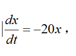
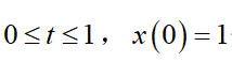
但是我們知道了它的初始條件,這對于我們疊代求解很有幫助,也是必須的�。
那么現(xiàn)在我們也用Python去解決這一些問題���,一般的數(shù)值解法有歐拉法��、隱式梯形法等,我們也來看看這些算法對疊代的精度有什么區(qū)別�����?
```python
```python
import numpy as np
from scipy.integrate import odeint
from matplotlib import pyplot as plt
import os
#先從odeint函數(shù)直接求解微分方程
#創(chuàng)建歐拉法的類
class Euler:
#構造方法�����,當創(chuàng)建對象的時候�����,自動執(zhí)行的函數(shù)
def __init__(self,h,y0):
#將對象與對象的屬性綁在一起
self.h = h
self.y0 = y0
self.y = y0
self.n = 1/self.h
self.x = 0
self.list = [1]
#歐拉法用list列表,其x用y疊加儲存
self.list2 = [1]
self.y1 = y0
#改進歐拉法用list2列表���,其x用y1疊加儲存
self.list3 = [1]
self.y2 = y0
#隱式梯形法用list3列表����,其x用y2疊加儲存
#歐拉法的算法���,算法返回t,x
def countall(self):
for i in range(int(self.n)):
y_dere = -20*self.list[i]
#歐拉法疊加量y_dere = -20 * x
y_dere2 = -20*self.list2[i] + 0.5*400*self.h*self.list2[i]
#改進歐拉法疊加量 y_dere2 = -20*x(k) + 0.5*400*delta_t*x(k)
y_dere3 = (1-10*self.h)*self.list3[i]/(1+10*self.h)
#隱式梯形法計算 y_dere3 = (1-10*delta_t)*x(k)/(1+10*delta_t)
self.y += self.h*y_dere
self.y1 += self.h*y_dere2
self.y2 =y_dere3
self.list.append(float("%.10f" %self.y))
self.list2.append(float("%.10f"%self.y1))
self.list3.append(float("%.10f"%self.y2))
return np.linspace(0,1,int(self.n+1)), self.list,self.list2,self.list3
step = input("請輸入你需要求解的步長:")
step = float(step)
work1 = Euler(step,1)
ax1,ay1,ay2,ay3 = work1.countall()
#畫圖工具plt
plt.figure(1)
plt.subplot(1,3,1)
plt.plot(ax1,ay1,'s-.',MarkerFaceColor = 'g')
plt.xlabel('橫坐標t',fontproperties = 'simHei',fontsize =20)
plt.ylabel('縱坐標x',fontproperties = 'simHei',fontsize =20)
plt.title('歐拉法求解微分線性方程步長為'+str(step),fontproperties = 'simHei',fontsize =20)
plt.subplot(1,3,2)
plt.plot(ax1,ay2,'s-.',MarkerFaceColor = 'r')
plt.xlabel('橫坐標t',fontproperties = 'simHei',fontsize =20)
plt.ylabel('縱坐標x',fontproperties = 'simHei',fontsize =20)
plt.title('改進歐拉法求解微分線性方程步長為'+str(step),fontproperties = 'simHei',fontsize =20)
plt.subplot(1,3,3)
plt.plot(ax1,ay3,'s-.',MarkerFaceColor = 'b')
plt.xlabel('橫坐標t',fontproperties = 'simHei',fontsize =20)
plt.ylabel('縱坐標x',fontproperties = 'simHei',fontsize =20)
plt.title('隱式梯形法求解微分線性方程步長為'+str(step),fontproperties = 'simHei',fontsize =20)
plt.figure(2)
plt.plot(ax1,ay1,ax1,ay2,ax1,ay3,'s-.',MarkerSize = 3)
plt.xlabel('橫坐標t',fontproperties = 'simHei',fontsize =20)
plt.ylabel('縱坐標x',fontproperties = 'simHei',fontsize =20)
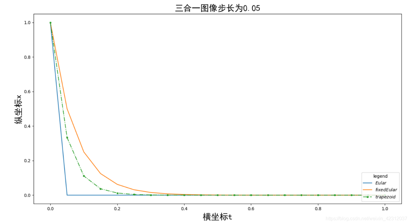
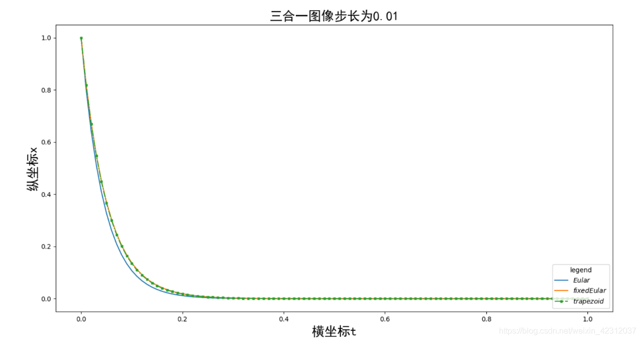
plt.title('三合一圖像步長為'+str(step),fontproperties = 'simHei',fontsize =20)
ax = plt.gca()
ax.legend(('$Eular$','$fixed Eular$','$trapezoid$'),loc = 'lower right',title = 'legend')
plt.show()
os.system("pause")
對于歐拉法,它的疊代方法是:
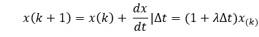
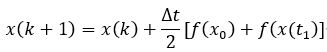
改進歐拉法的疊代方法:

隱式梯形法:
對于不同的步長,其求解的精度也會有很大的不同�����,我先放一幾張結果圖:
補充:基于python的微分方程數(shù)值解法求解電路模型
安裝環(huán)境包
安裝numpy(用于調節(jié)range) 和 matplotlib(用于繪圖)
在命令行輸入
pip install numpy
pip install matplotlib
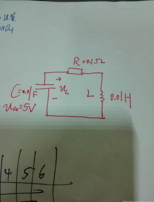
電路模型和微分方程
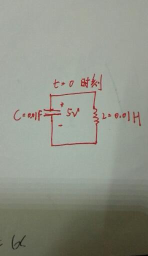
模型1
無損害��,電容電壓為5V�����,電容為0.01F�����,電感為0.01H的并聯(lián)諧振電路
電路模型1
微分方程1
模型2
帶電阻損耗的電容電壓為5V,電容為0.01F��,電感為0.01H的的并聯(lián)諧振
電路模型2
微分方程2
python代碼
模型1
import numpy as np
import matplotlib.pyplot as plt

L = 0.01  #電容的值 F
C = 0.01  #電感的值 L
u_0 = 5   #電容的初始電壓
u_dot_0 = 0

def equition(u,u_dot):#二階方程
    u_double_dot = -u/(L*C)
    return u_double_dot

def draw_plot(time_step,time_scale):#時間步長和范圍
    u = u_0
    u_dot = u_dot_0  #初始電壓和電壓的一階導數(shù)
    time_list = [0] #時間lis
    Votage = [u] #電壓list
    plt.figure()
    for time in np.arange(0,time_scale,time_step):#使用歐拉數(shù)值計算法 一階近似
        u_double_dot = equition(u,u_dot) #二階導數(shù)
        u_dot = u_dot + u_double_dot*time_step #一階導數(shù)
        u = u + u_dot*time_step #電壓
        time_list.append(time) #結果添加
        Votage.append(u) #結果添加
        print(u)
    plt.plot(time_list,Votage,"b--",linewidth=1) #畫圖
    plt.show()
    plt.savefig("easyplot.png")

if __name__ == '__main__':
    draw_plot(0.0001,1)
模型2
import numpy as np
import matplotlib.pyplot as plt

L = 0.01  #電容的值 F
C = 0.01  #電感的值 L
R = 0.1   #電阻值
u_0 = 5   #電容的初始電壓
u_dot_0 = 0

def equition(u,u_dot):#二階方程
    u_double_dot =(-R*C*u_dot -u)/(L*C)
    return u_double_dot

def draw_plot(time_step,time_scale):#時間步長和范圍
    u = u_0
    u_dot = u_dot_0  #初始電壓和電壓的一階導數(shù)
    time_list = [0] #時間lis
    Votage = [u] #電壓list
    plt.figure()
    for time in np.arange(0,time_scale,time_step):#使用歐拉數(shù)值計算法 一階近似
        u_double_dot = equition(u,u_dot) #二階導數(shù)
        u_dot = u_dot + u_double_dot*time_step #一階導數(shù)
        u = u + u_dot*time_step #電壓
        time_list.append(time) #結果添加
        Votage.append(u) #結果添加
        print(u)
    plt.plot(time_list,Votage,"b-",linewidth=1) #畫圖
    plt.show()
    plt.savefig("result.png")

if __name__ == '__main__':
    draw_plot(0.0001,1)
數(shù)值解結果
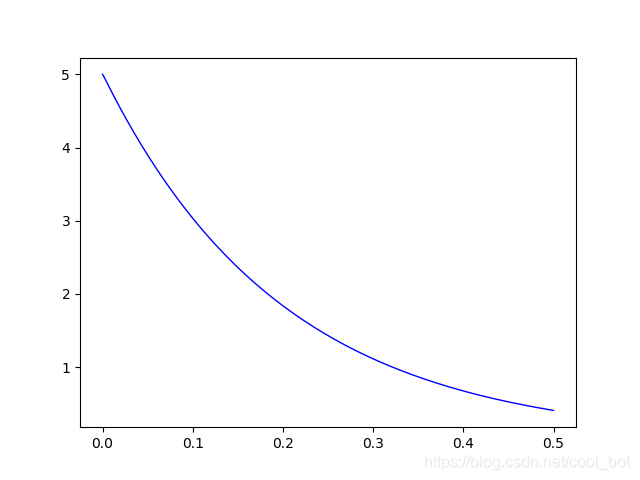
模型1
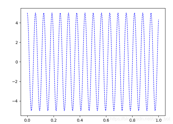
縱軸為電容兩端電壓�����,橫軸為時間與公式計算一致
模型2結果
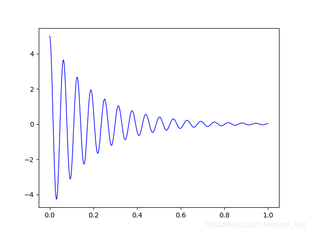
縱軸
為電容兩端電壓,橫軸為時間標題
最后我們可以根據(jù)調節(jié)電阻到達不同的狀態(tài)

R=0.01����,欠阻尼
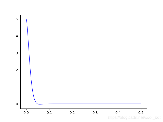
R=1.7,臨界阻尼
R=100,過阻尼
以上為個人經驗,希望能給大家一個參考�����,也希望大家多多支持腳本之家����。
您可能感興趣的文章:- python實現(xiàn)各種插值法(數(shù)值分析)
- python實現(xiàn)數(shù)值積分的Simpson方法實例分析
- Python導入數(shù)值型Excel數(shù)據(jù)并生成矩陣操作
- Python實現(xiàn)列表中非負數(shù)保留,負數(shù)轉化為指定的數(shù)值方式
- 使用Python matplotlib作圖時,設置橫縱坐標軸數(shù)值以百分比(%)顯示
- Python如何將函數(shù)值賦給變量
- 教你如何利用python進行數(shù)值分析